Brain Tumor Classification with NVIDIA TAO Toolkit

In this tutorial, we will walk through the process of brain tumor classification using the NVIDIA TAO Toolkit. Previously, we mentioned No-Code AI Model Training with TAO Toolkit and How to Install NVIDIA TAO Toolkit.

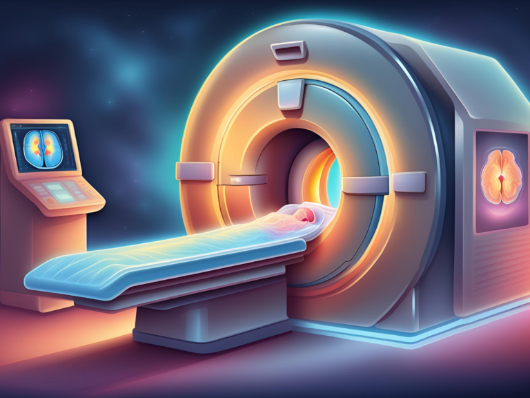
Brain tumor classification from MRI (Magnetic Resonance Imaging) images is crucial in medical diagnostics. Automated and accurate classification can assist radiologists in diagnosing and categorizing tumors, which aids in deciding appropriate treatment regimens. 

NVIDIA TAO Toolkit offers developers, data scientists, and researchers a platform to build AI models for various applications, including medical imaging. This tutorial will mention how to classify brain tumors using the TAO Toolkit.

This dataset and tutorial is not prepared for diagnostic usage! The aim is demonstrating features of TAO Toolkit in medical imaging.

Model Training Steps

1. Preparing TAO Environment
2. Preparing MRI Brain Tumor Classification Dataset
3. Model Configuration
4. Model Training
5. Model Evaluation

Preparing TAO Toolkit Environment

We mentioned How to Install the NVIDIA TAO Toolkit. Before. Be sure you have installed the TAO Toolkit and pulled the TAO Toolkit PyTorch Docker Image because we will use the TAO Toolkit with PyTorch backend. You don’t need to create a new container from the image. TAO Python package handles all this stuff for us.

Project Folder Structure

Create a folder TAO in your home directory. We will mount this folder to our TAO container in the next step, and then this folder will be common in both our system and the container.

Create a brain-tumor-classification folder in the TAO folder. This will be our main project folder for this tutorial. We will store our dataset, experiments, checkpoints, and configuration files in this folder. It is a good practice to separate project structures like these.

TAO Mounts JSON File Configuration

We should create and configure .tao_mounts.json file in our home directory. TAO automatically mounts these folders to our TAO containers. So, our local files will be accessible from the containers.

Let’s create a .tao_mounts.json file using nano.

nano ~/.tao_mounts.json

Then, define our source and destination folders like below. Be aware that, the source is the local path, the destination is the container path. In other words, /tao-workspace is an alias of /home/aaslan/Workspace/TAO folder in the container.

{
    "Mounts": [
        {
            "source": "/home/aaslan/Workspace/TAO",
            "destination": "/tao-workspace"
        }
    ]
}

Save and exit from nano. The TAO folder is accessible from the container now.

Preparing Brain Tumor Classification Dataset

We will use this paper’s dataset in this tutorial. These images have been meticulously cleaned and augmented to bolster the dataset’s robustness and potentially enhance the performance of deep learning models trained on it. The dataset is specifically curated to identify and subsequently classify brain tumors from MRI scans. 

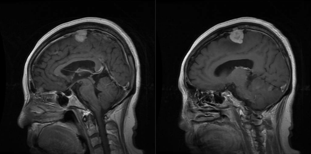
The dataset has four classes, allowing for the differentiation between Benign Tumors, Malignant Tumors, Pituitary Tumors, and No Tumors. It comprises 3,260 T1-weighted contrast-enhanced images, a preferred modality in radiology for distinguishing pathological tissues. The dataset is ~92MB, and every image is in a PNG format with 512x512px dimensions. Also, the dataset has already been split into training and test sets.

Go to the brain-tumor-classification folder and pull the dataset. This command will download the dataset to the dataset folder.

git clone https://github.com/SartajBhuvaji/Brain-Tumor-Classification-DataSet/ dataset

Create a classes.txt file in the brain-tumor-classification folder and write a class name for each line in the dataset.

nano classes.txt

classes.txt file should look like this. Save and exit.

glioma_tumor
meningioma_tumor
no_tumor
pituitary_tumor

Model Configuration

In TAO, we configure our models using YAML configuration files. These files ensure that we configure our brain tumor classification model without any Python coding end-to-end. Also, we can easily try different configurations without a hassle. Training, evaluation, and export processes can have different configurations. Now, we will create only a configuration for training. 

If you don’t know anything about YAML file you can read this tutorial prepared by RedHat.

Create a config.yaml file in the brain-tumor-classification folder using nano. We will store our model configurations here.

nano config.yaml

Then copy and paste this configuration and save it. 

train:
  exp_config:
    manual_seed: 42
  train_config:
    runner:
      max_epochs: 100
    checkpoint_config:
      interval: 1
    logging:
      interval: 500
    validate: True
    evaluation:
      interval: 1
dataset:
  data:
    samples_per_gpu: 32
    train:
      data_prefix: /tao-workspace/brain-tumor-classification/dataset/Training/
      pipeline: 
        - type: RandomResizedCrop
          size: 224
      classes: /tao-workspace/brain-tumor-classification/classes.txt
    val:
      data_prefix: /tao-workspace/brain-tumor-classification/dataset/Testing/
      classes: /tao-workspace/brain-tumor-classification/classes.txt
    test:
      data_prefix: /tao-workspace/brain-tumor-classification/dataset/Testing/
      classes: /tao-workspace/brain-tumor-classification/classes.txt
model:
  backbone:
    type: "fan_tiny_8_p4_hybrid"
    custom_args:
      drop_path: 0.1
  head:
    num_classes: 4
    loss:
      type: "CrossEntropyLoss"

Training Settings (train):

• Experiment Configuration (exp_config):
  • manual_seed: The random seed is set to 42. Setting a seed ensures reproducibility. This means that every time you run the model with this configuration, the random processes (like data shuffling) will be the same.
• Training Configuration (train_config):
  • runner:
    • max_epochs: The model will be trained for 100 epochs. An epoch is one complete forward and backward pass of all the training examples.
  • checkpoint_config:
    • interval: A model checkpoint will be saved every one epoch.
  • logging:
    • interval: Logging information will be saved or printed every 500 training iterations.
  • validate: It’s set to True, meaning the model will be validated during training.
  • evaluation:
    • interval: Evaluation will be performed every one epoch.

Dataset Configuration (dataset):

• data:
  • samples_per_gpu: For each GPU, 32 samples will be loaded.
• Training Data (train):
  • data_prefix: Specifies the directory path to the training dataset.
  • pipeline: Defines data augmentation/preprocessing steps.
    • RandomResizedCrop: The images will be randomly cropped and resized to 224×224 pixels.
  • classes: Specifies the path to the file containing the class labels.
• Validation Data (val):
  • data_prefix: Specifies the directory path to the validation dataset.
  • classes: Specifies the path to the file containing the class labels.
• Testing Data (test):
  • data_prefix: Specifies the directory path to the test dataset.
  • classes: Specifies the path to the file containing the class labels.

Model Configuration (model):

• Backbone Configuration (backbone):
  • type: Specifies the type of the model backbone, which is “fan_tiny_8_p4_hybrid”.
  • custom_args:
    • drop_path: Specifies a drop path rate of 0.1, a form of regularization to prevent overfitting.
• Head Configuration (head):
  • num_classes: The model is expected to be classified into four different classes.
  • loss: Specifies the type of loss function the model will use, “CrossEntropyLoss”. This is a common loss function for classification tasks.

You can learn further information about the configurations from the Image Classification PyT documentation.

Model Training

Create an experiments folder in the brain-tumor-classification folder. We will store our model checkpoints in this folder.

Before starting the training process, our folder structure should look like this.

brain-tumor-classification
├── dataset
│   ├── Testing
│   │   ├── glioma_tumor
│   │   ├── meningioma_tumor
│   │   ├── no_tumor
│   │   └── pituitary_tumor
│   └── Training
│       ├── glioma_tumor
│       ├── meningioma_tumor
│       ├── no_tumor
│       └── pituitary_tumor
├── experiments
└── config.yaml
└── classes.txt

If all configurations and files are ready, we can start training!

tao model classification_pyt train -e /tao-workspace/brain-tumor-classification/config.yaml -r /tao-workspace/brain-tumor-classification/experiments

This command instructs the TAO Toolkit to train a PyTorch-based classification model using the configurations provided in the config.yaml file and save the results of this training experiment in the specified directory. Please note that all paths in this command are based on the container, not our local file system.

After the command, TAO will create a container, load the model structure, and start training. You can monitor the training process from the command line. Training will end after the 100th epoch, as we set in the config.yaml file. Also, all model checkpoints will be in the experiments/train folder.

Model Evaluation

We can evaluate our brain tumor classification model when the training process is finished. Again, we can evaluate the model TAO package from the command line.

tao model classification_pyt evaluate -e /tao-workspace/brain-tumor-classification/config.yaml evaluate.checkpoint=/tao-workspace/brain-tumor-classification/experiments/train/epoch_23.pth results_dir=/tao-workspace/brain-tumor-classification/results

This command evaluates a specific PyTorch-based classification model checkpoint using the provided configuration and saves the evaluation results to the designated directory. Task-specific results will also be prompted to the terminal.

Conclusion

In conclusion, the NVIDIA TAO Toolkit stands out as a remarkably efficient tool for training and evaluating deep learning models. Our ability to achieve these results is astonishing without writing a single line of Python code. This speaks to the toolkit’s user-friendly nature and showcases its potential to democratize AI by making it accessible to a wider range of users. 

We will mention optimizing and deploying models in upcoming posts.